Supply and Demand

Overview

What is Economy?

Economy: Economy is a science that studies the set of actions and choices individuals, businesses, communities and government take as a result some set of incentives and scarcities.

Demand and Supply

Demand

For a product or service to have demand there must be 3 criterion that must be met:

A) You must want it.
B) You must be able to afford this product or service
C) You must have a plan to purchase this product or service

People usually have infinite desires and wants but most fail to meet B) and C) and so their demand is diminished. This concept is best summarised by the Law of Demand.

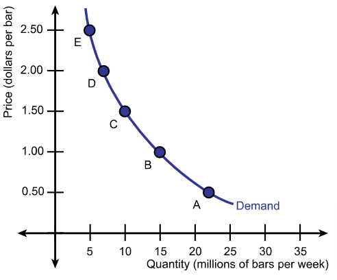
Law of Demand: The higher the price of a product of service, the smaller the quantity demanded. Likewise, the lower the price of a good the higher the demand.

The law of demand occurs because of two reasons:

A) Substitution Effect: When a price of a good increases, the relative price against competitors selling the same good increases. Once the price of the good exceeds competitor’s price, the public has more incentive to purchase goods from competitors than from you.
B) Income Effect: When a price of a good increases, the quantity of the good a consumer can purchase decreases due to their fixed income.

If you have $x$ dollars to purchase some quantity $q$ of the good, the cost per $1$ quantity is $\frac{x}{q}$. There is a inverse relationship between the price and quantity. Using this we can define the demand curve where as the quantity increases the price per 1 quantity of good decreases:

There are a set of things that may impact the demand curve:

1. Prices of Related Goods: For a given good we have substitute and complements. Substitutes are alternatives to a given good, like Mustard and Ketchup. If a substitutes price decreases, the demand for your good decreases and vise-versa. Likewise a complement is a set of goods that are needed together, like hot dog buns and Ketchup. If the demand for a good A increases the demand for all the complements for good A also increases and vise-versa.
2. Expected Future Prices: If prices are expected to rise in the future the current demand for that good would also increase. Real estate investment works in a similar fashion.
3. Income: Demand quantity increases when income of individuals increases. The demand curve shifts right. We can have 2 types of good. Normal Goods, whose quantity demanded increases when income increases. Inferior good whose quantity demanded decreases when income increases.

If demand for a particular good increases, the demand curve shifts rightward. Likewise, if the demand of the good decreases, the graph shifts leftward.

Supply

There are 3 criterion that a firm must meed in order to be a supplier of a good:

A) Must have resources to produce a given good/service
B) Must be profitable from producing the good/service
C) Must have a definite plan to produce the good/service

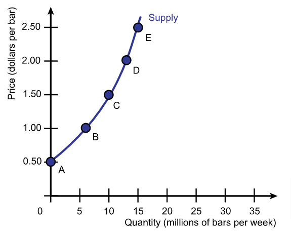
Law of Supply: The higher the price of a good the larger the quantity supplied will be. Likewise, the smaller the price of the good the smaller the quantity supplied will be.

This law may seem counter intuitive, especially since the higher the price of the good the smaller the demand for the good. So, how come the supply increases? To understand this, we must understand marginal cost.

Marginal Cost: is the change in production cost resulting from producing one more unit of a good or service. $$ \text{Marginal Cost of Production}=\frac{\text{Change in total Production Costs}}{\text{Change in total Quantity Produced}} $$ Marginal costs of production will keep going down as production rises until the company needs to incur more costs tor produce more products.

Therefore, from the eyes of the producer the higher the cost of the good or service, the lower the marginal cost of producing one more unit of that good. Therefore, more of that good can be produced as compared to a cheaper good.

A supply curve displays the relationship between quantity supplied and the price of the good. From the law of supply the higher the cost of a good the more that can be supplied due to the low marginal costs.

When supply of a particular curve increases, the supply curve shifts right. Likewise, when the supply decreases, the supply curve shifts left.

There are a set of things that may impact the supply curve:

1. The Prices of Factors of Production: If the price of a factor of production rises, the cost of selling a good also rises, but the price that the producer can sell for remains the same. The producer in this case must produce less, thereby decreasing the supply.
2. The Prices of Related Goods Produced: For a substitute in production if the price of a related good increases, the producer will switch to the related good in order to secure the higher profits. Thus supply of a good or service will decrease when the price of a substitute rises, the supply curve shifts left.
3. Expected Future Prices: if the price of a good rises in the near future the supplier will want to sell the good in the near future to secure higher profits. The supply curve will decrease, since the producer will sell later.
4. The Number of Suppliers: More suppliers, more goods. Thus the supply curve shifts rightward.

Market Equilibrium

In a global market place we have transactions between buyers and sellers. To see at which price these interactions take place we can see the price demanded for a quantity demanded vs price asked for a quantity supplied. This created an equilibrium point at which both buyers and sellers agree for an exchange.

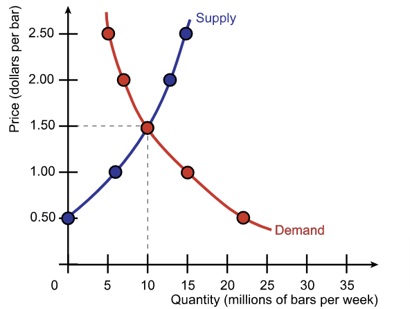
The market will always approach the equilibrium. For example if the price is too high, say $2.00 from the above diagram, the quantity demanded will be 7 units where as the quantity supplied will be 13 units. Thus there is a surplus of the good. Producers don’t want any surplus, therefore they will reduce the price which will in turn increase the demand. Thus reaching the equilibrium. On the other hand, if the price is too low, say $1.00 from the above diagram, the quantity demanded will 15 whereas the quantity supplied will be 5. Thus there is a shortage of 10. Suppliers do not want a shortage. Thus they will increase the price, thereby decreasing the demand and this again continues until equilibrium is achieved.

If we know the equation for the supply and demand curve we can solve for the equilibrium

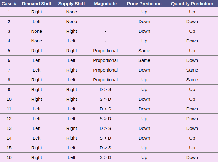
Predicted changes in Price and Quantity

We can have shifts to the supply and demand curve, each in turn resulting in Price and Quantity changes at the equilibrium. The possible outcomes are summarized below:

Elasticity

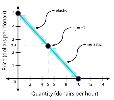
Elasticity- The magnitude of change in price due to demand/supply curve shift

Elasticity of Demand

Measure of the responsiveness of the quantity demanded of a good to a change in its price

The elasticity of demand is given by the following formula, where $Q$ is the quantity and $P$ is the price: $$ \epsilon_D = \frac{\frac{\Delta Q}{\bar{Q}}}{\frac{\Delta P}{\bar{P}}} $$

• Note $\Delta A = A_{new}-A_{old}$ and $\bar{A} = \text{Average($A$)}$
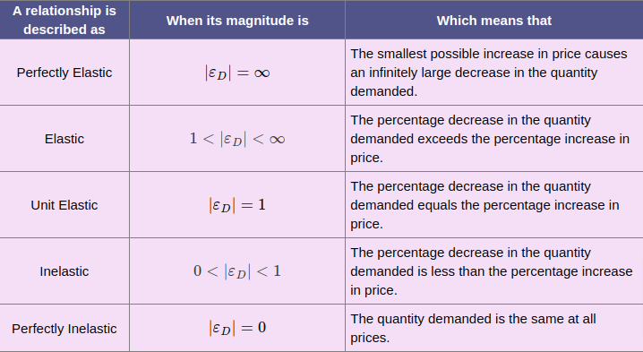
• $\epsilon_D=0 \implies$ demand is Perfectly Inelastic
• $\epsilon_D=-1 \implies$ demand is Unit Elastic
• $\epsilon_D < 1 \implies$ demand is Inelastic
• $\epsilon_D>1 \implies$ demand is Elastic
• $\epsilon_D=\infty \implies$ demand is Perfectly Elastic (division by 0)

From the suppliers point of view the revenue is directly related to a price of good, so elasticity directly effects the revenue. If demand is elastic, 1% price cut results in quantity sold increasing by more than 1%, thus total revenue increases. If demand is inelastic, a 1% price cut increases the quantity sold by less than 1%, total revenue decreases. If the demand is unit elastic, a 1% price cut result in increasing quantity sold by 1%, and the total revenue is unchanged.

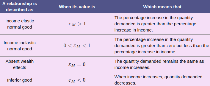
Income Elasticity of Demand

Measure the responsiveness of quantity demanded of a good to some change in consumer income.

The income elasticity of demand is given by the following formula, where $Q$ is the quantity and $I$ is the income: $$ \epsilon_M = \frac{\frac{\Delta Q}{\bar{Q}}}{\frac{\Delta I}{\bar{I}}} $$

• If $\epsilon_M > 1 \implies$ demand is income elastic & good being bought is normal good
• If $0 < \epsilon_M < 1 \implies$ demand is income inelastic & good being bought is again a normal good
• If $\epsilon_M < 0 \implies$ good good being bought is an inferior good

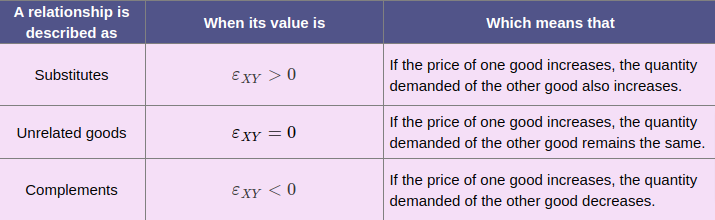
Cross Elasticity of Demand

Measurement of the responsiveness of the quantity demanded of a good to a change in the price of a substitute or a complement

The cross elasticity of demand is given by the following formula, where $Q$ is the quantity, $P$ is the price, $X$ is one type of good (good $X$) and $Y$ is another type of good (good $Y$): $$ \epsilon_{XY} = \frac{\frac{\Delta Q^X}{\bar{Q^X}}}{\frac{\Delta P^Y}{\bar{P^Y}}} $$

• if $\epsilon > 0 \implies$ $X$ and $Y$ are substitutes
• if $\epsilon < 0 \implies$ $X$ and $Y$ are complements

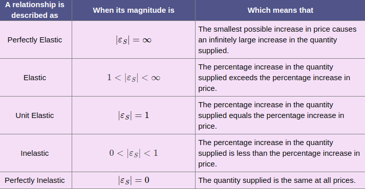
Elasticity of Supply

Measurement for the responsiveness of a quantity supplied of a good to a change in its price

The elasticity of supply is given by the following formula, where $Q$ is the quantity and $P$ is the price: $$ \epsilon_S = \frac{\frac{\Delta Q}{\bar{Q}}}{\frac{\Delta P}{\bar{P}}} $$

• If $\epsilon_S = 0 \implies$ perfectly inelastic
• If $0 < \epsilon_S < 1 \implies$ inelastic
• If $\epsilon_S = 1 \implies$ unit elastic
• If $\epsilon_S > 1 \implies$ elastic
• If $\epsilon_S = \infty \implies$ perfectly elastic

Efficiency and Equity

Consumer Surplus

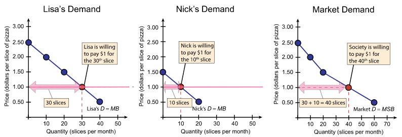
To understand consumer surplus, we first need to understand the notion of a market demand curve. Market demand curve is the demand curve which represents the quantity demanded by the entire market rather than demands of individuals:

Consumer surplus is defined as the excess of benefit received from a good or service over the amount paid for the good or service. For instance, if you find a bike for which you are willing to pay $100 but there is a deal which allows you to purchase the bike for $50. Your receive a surplus of $50 which is what you saved off of the transaction.

For the following graph, we can compute the consumer surplus as follows:

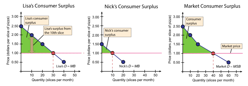$$ \text{Lisa’s consumer surplus} = \frac{1}{2}\times30\times1.50 $$

• Note that both the height and base of the triangle effect the consumer surplus. Increasing the price will decrease the quantity, thereby decreasing the consumer surplus.

To find the market surplus we must sum the surplus of Lisa and Nick. Generally, we would sum the surplus of all consumers in a given market place to obtain the market surplus.

Producer Surplus

We can start by defined the market supply curve as we did with market demand curve. Market supply curve is the sum on quantities that each supplier can supply at a given price:

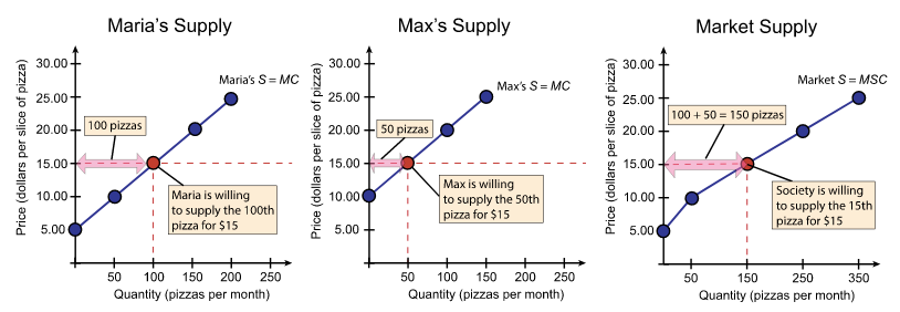
Likewise, when the price of a good exceeds the price of producing the good. That is referred to as the producer surplus.

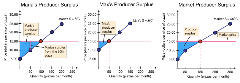
Once again, we can compute the producer surplus by computing the area under the market price. For example, Maria’s producer surplus is: $$ \text{Maria’s consumer surplus} = \frac{1}{2}\times100\times10 $$ The market producer surplus is the sum of the surplus for all the producers.

Competitive Equilibrium and Efficiency

Again, we can find the market equilibrium by overlaying market supply curve with the market demand curve. Now we can identify the consumer and producer surplus:

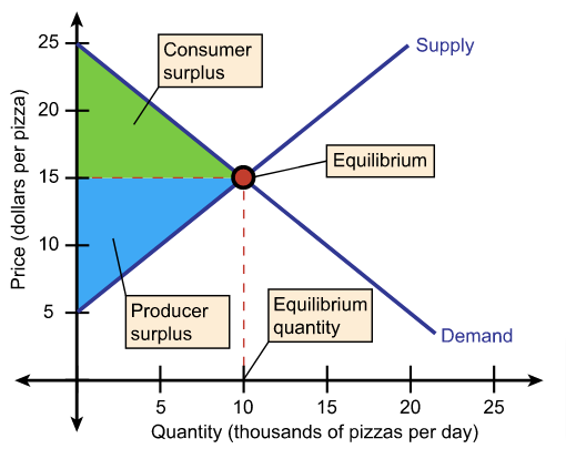
We can define the concept of Total Surplus:
$\text{Total Surplus} = \text{Consumer Surplus} + \text{Producer Surplus}$

For the market in the image, the total surplus is maximised as the consumers and producers are receiving the greatest possible value at the market equilibrium.

Market Failures

A market failure is when a good is under or overproduced such that equilibrium is not met. Consider the following:

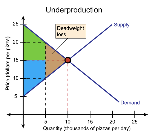
1. The market is producing fewer pizzas than the equilibrium
2. Consumer and producer surplus shrinks
3. Marginal Social Benefit > Marginal Social Cost
4. Since equilibrium is not met a dead-weight loss is produced

Dead-weight Lost is the decrease in total surplus

For over production we can similar situation:

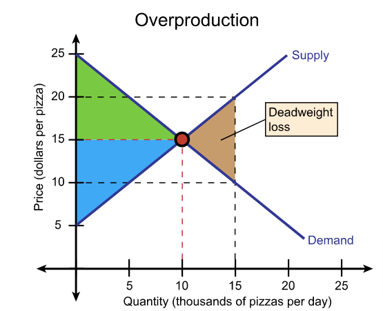
1. Market is producing more pizzas than needed priced at a higher price (because producers are incurring marginal costs of producing more pizzas) thus reducing the demand
2. Resources are being wasted in producing the extra pizzas
3. Marginal Social Benefit < Marginal Social Cost
4. Since equilibrium is not met a dead-weight loss occurs

Market failures can arise in many different situatations:

• Price and Quantity Regulation
• Taxes and subsidies
• Externalities
• Monopoly
• High Transactions Costs

Social Welfare

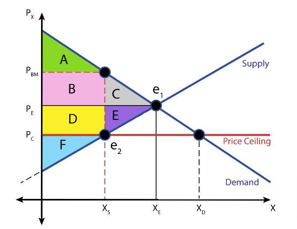
Price Ceilings

A regulation that makes it illegal to charge a price higher than a specific level

• if $\text{ceiling} > \text{Price} \implies$ there is no public effect
• if $\text{ceiling} < \text{Price} \implies$
  • A shortage (demand > supply)
  • Increased searching for good/service
  • Black market

Black Market - is an illegal market that operates alongside legal market in which a ceiling exists

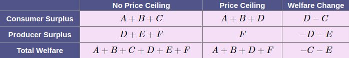
Market failures can result from a ceiling if ceiling < Price:

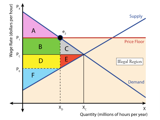
Price Floors

Regulation that makes it illegal to trade a price lower than a specific level. (Ex. Minimum Wage)

• if $\text{floor} < \text{Price} \implies$ there is no public effect
• if $\text{floor} > \text{Price} \implies$
  • A surplus occurs (supply > demand)
  • In the example of labour and minimum wage, unemployment would occur

Market failures can result from a floor if floor > price:

Production Quotas and Subsidies

Production Quota: upper limit to quantity of good that may be produced during some period of time

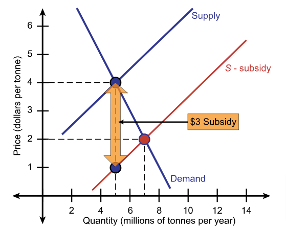
Subsidy: Payment made from a government to a producer

If a production quota < equilibrium quantity:

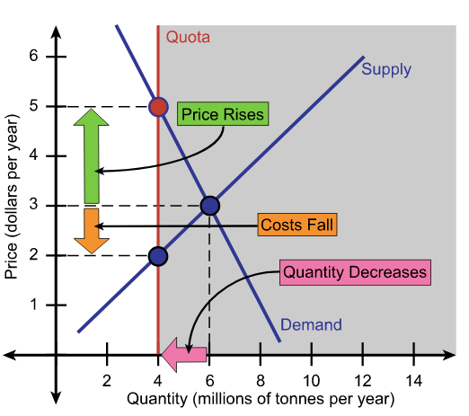
• Production is insufficient and producers have an incentive to cheat and provide for the excess demand

Subsidies on the other hand reduce the cost of production allowing producers to supply good with a lower price:

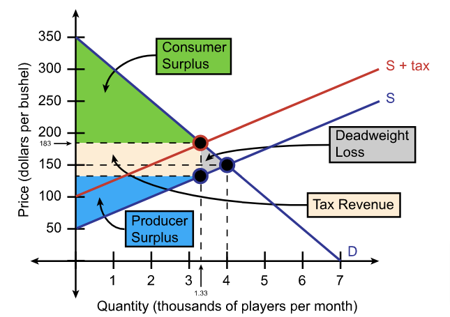
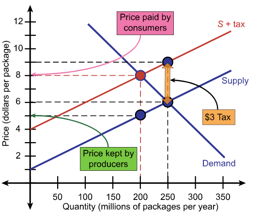
Taxes

Taxing the sellers often increase the price of producing a good:

Taxing the buyers often decreases the demand:

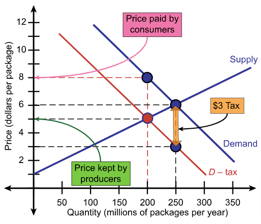
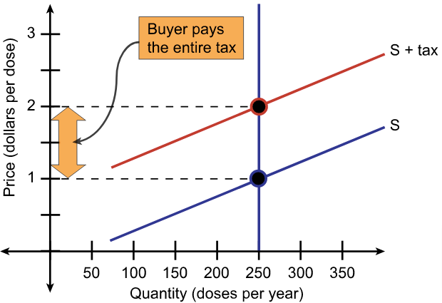
• Perfectly inelastic demand - Buyers pay the entire tax

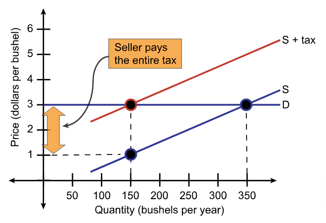
• Perfectly elastic demand- Sellers pay the entire tax

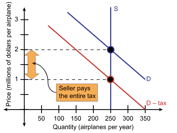
• Perfectly inelastic supply - Sellers pay the entire tax

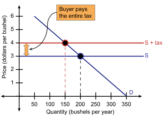
• Perfectly elastic supply - Buyers pay the entire tax

• Taxes can also result in deadweight loss, since the tax revenue takes part of the total surplus

• ← Previous Post
• Next Post →