Reviewing SQL

A Brief Review of SQL Queries

SELECT <columns>
FROM <table>
WHERE <predicate>
GROUP BY <columns>
HAVING <predicate>
ORDER BY <columns>
LIMIT <num>;

We have the following $7$ basic operations when querying data from a single table. We need to SELECT certain columns FROM a table, keep rows WHERE a certain condition matches. Potentially, GROUP columns that HAVE another condition matching (within the groups) and aggregate those results using aggregation functions. We can also ORDER BY one or more columns. Finally, LIMIT the number of results that are returned. If you are confused, you can find a more detailed explanation here

Reviewing Joins

We have these 6 basic joins:

1. Cross Join

Which is essentially the cartesian product of the two tables or in other words, every possible permutation of records from the first table with the records from the second table. The basic syntax is as follows:

select * from tableA, tableB;

2. Inner Join

Inner join is used to match records from two tables where one column in both records is an exact match. Although this notation is not heavily used in practice we could use the Cross Join to create the inner join query as follows:

select * from tableA, tableB
where colA = colB

In practice this next notation is a lot more common:

select * from tableA
inner join tableB
on colA = colB;

3. Left Outer Join

One drawback of the inner join is that records in either table that do not have a matching column in the opposite table are dropped. In some situations, we want all records in the left table and if their join doesn’t exist in the right table, just join it with a null record.

select * from leftTable
left outer join rightTable
on leftCol = rightCol;

This will ensure all records from the left table exist and if the matching record in the right table is not found. We will simply append NULL values for the remaining columns.

4. Right Outer Join

Simply the opposite of the Left Outer Join, where we want to keep every record in the right table and if the matching column does not exist in the left table we simply append NULL values for all the left record columns.

select * from leftTable
right outer join rightTable
on leftCol = rightCol;

5. Full Outer Join

Full outer join performs both left outer join and right outer join and displays the unique records. This means will find both left and right records at least once and if the match is not found in either the left or right table, we will simply append NULL values in that table.

select * from leftTable
full outer join rightTable
on leftCol = rightCol;

6. Natural Join

Natural join will simply join the first column that has the same name in both tables. Therefore, we don’t require the on clause in the query:

select * from leftTable
natural join rightTable;

Reviewing Sub-Queries

If you have to query data that requires multiple steps. For example, select classes that have a higher than the average number of students from all offered classes. This query requires us to determine the average number of students and find classes that have students larger than that value. In this situation, sub-queries come in very handy. You can use this very helpful page to review different types of sub-queries to refresh your memory.

Where Sub-Queries

select num from enrollment
where students >= (
    select avg(students) from enrollment
);

Correlated Sub-Queries

select * from classes
where exists (
    select * from enrollment
    where classes.num = enrollment.num
);

Sub-Queries from a FROM

select * from (
    select num from classes
) as a
where num = 'CS340';

Sub-Queries Factoring

with course_enrollment as (
    select * from courses
    natural join enrollment
);

select * from course_enrollment;

Lets talk about Storage

Now data needs to be stored somewhere and in a manner such that it can be easily read and written. Current technology offers several tiers of storage in increasing speed but decreasing size:

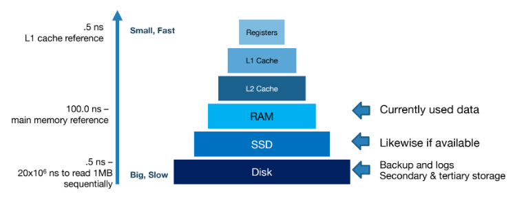
Disks

The reason disks are slow is because we need to spin the disk head into place and rotate the disk to the right position. The former can take 2-3ms on average and the latter can take up to 0-4ms with a 15,000 RPM motor. Now the transfer time is highly dependent on locality, if the memory being saught is contiguous then 0.25ms to read 64KB. Now this is awful compared to cache memory which can retrieve data within ns.

SSD

Now the power-off SSD is that it offers comparably fast random read times. However, the drawback is storage cells tend to wear out. This is combated by using wear leveling which ensures that writes are randomized so no one cell wears out too quickly.

How DB Data is stored

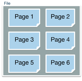
A table/relation consists of rows which are referred to as records, these records are organized into pages. A page is the smallest block of data that can be transferred from disk to main memory or can be written from main memory to disk. Now for data to be persisted it needs to be stored in the form of a file. Therefore, files will contain pages, which consist of records that belong to the same relation.

SQL employs internal algorithms to select the most cost-effective strategy for executing queries. The cost is measured based on the number of disk pages that have to be written or read during the query. This is because I/O operations can be expensive because they force us to interact with the disk, thus it is important to minimize these operations.

Records

There are 2 types of records, Fixed Length Records and Variable Length Records. This difference in types is due to the fact we can have fixed length types like int, and we can also have variable length types like varchar.

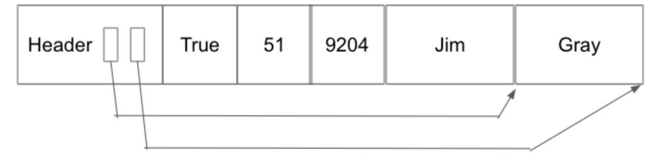
The above diagram shows how different data types are stored. The datum stores different fixed-length fields after the header. The header stores pointers to the start and end of variable length fields.

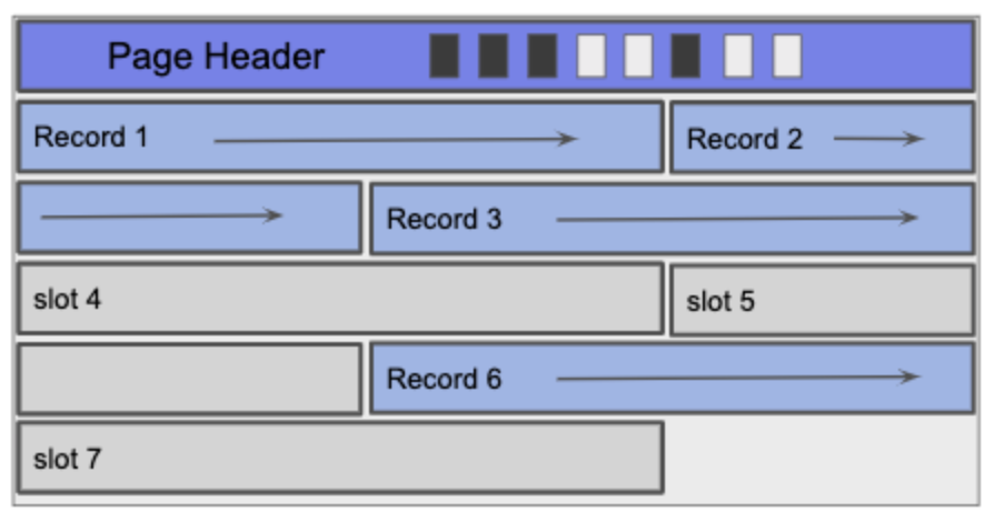
Pages

As mentioned before multiple records are stored on pages and there are two types of pages. There are pages to handle fixed-length records and variable-length records. Let us discuss pages for fixed-length records first. The page header stores the size of the records and the number of records that are currently stored. We can use both these pieces to find the position of the insertions. Deletion makes things tricker because it leaves empty record slots that could be filled with newer records. The way this is handled is by having a bitmap that stores which slots are empty and this way during insertion we can first check the bitmap to fill in empty slots before appending to the end of the page.

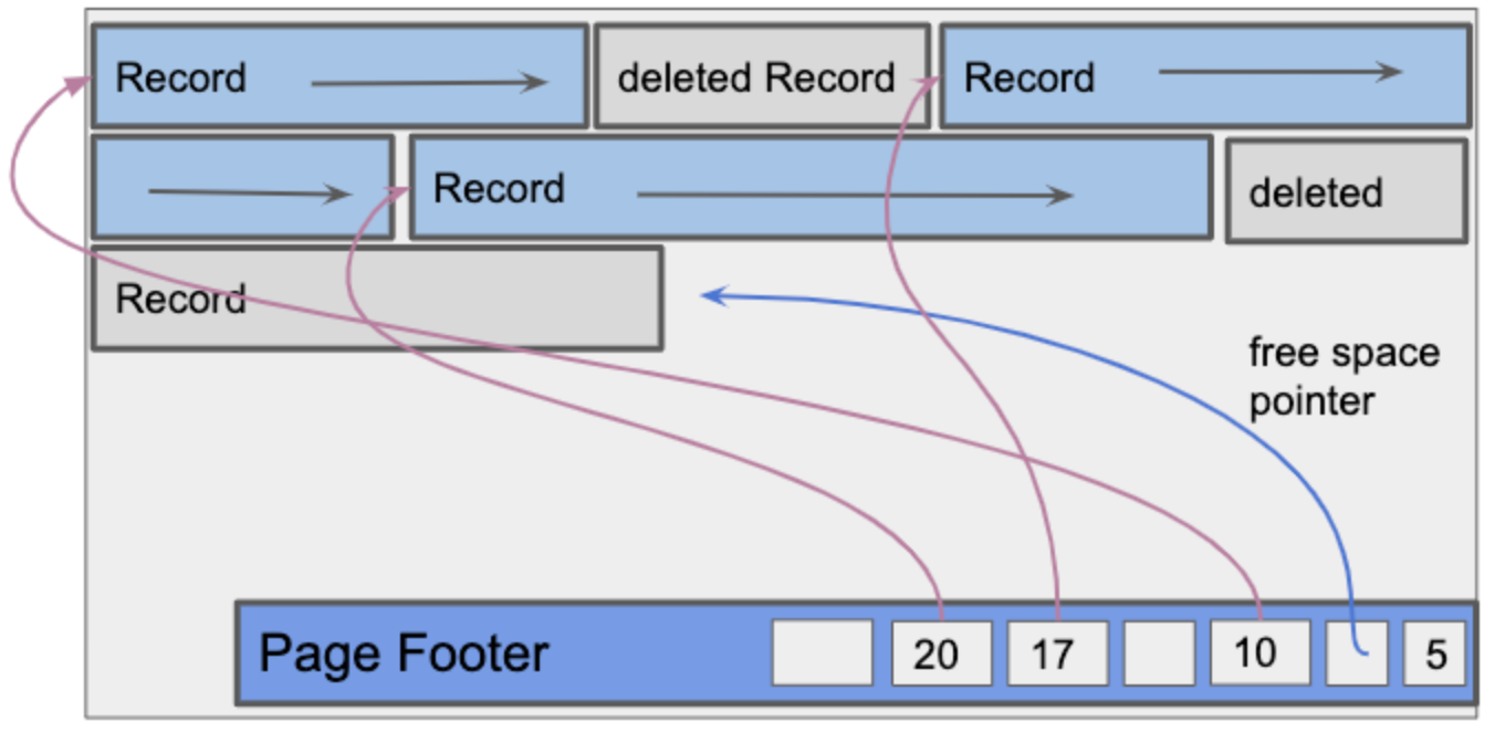
Dealing with pages for variable-length records is more tricky. The tricky bit is since we do not know beforehand how many records will be stored on the page we cannot perform the previous computations for insertion. Additionally, cannot know the size of the bitmap because the number of records is variable. Both these complexities require a dynamic-sized header. However, to avoid adjusting the data we should instead have a footer that grows upward. This footer will store pointers to free space for new insertions, pointers for deletion space and pointers for existing records. This can be stored in a [pointer, size] format. Using this footer, periodically records will be reorganized for compaction. To ensure that the deleted space can be converted to free space.

Indexes

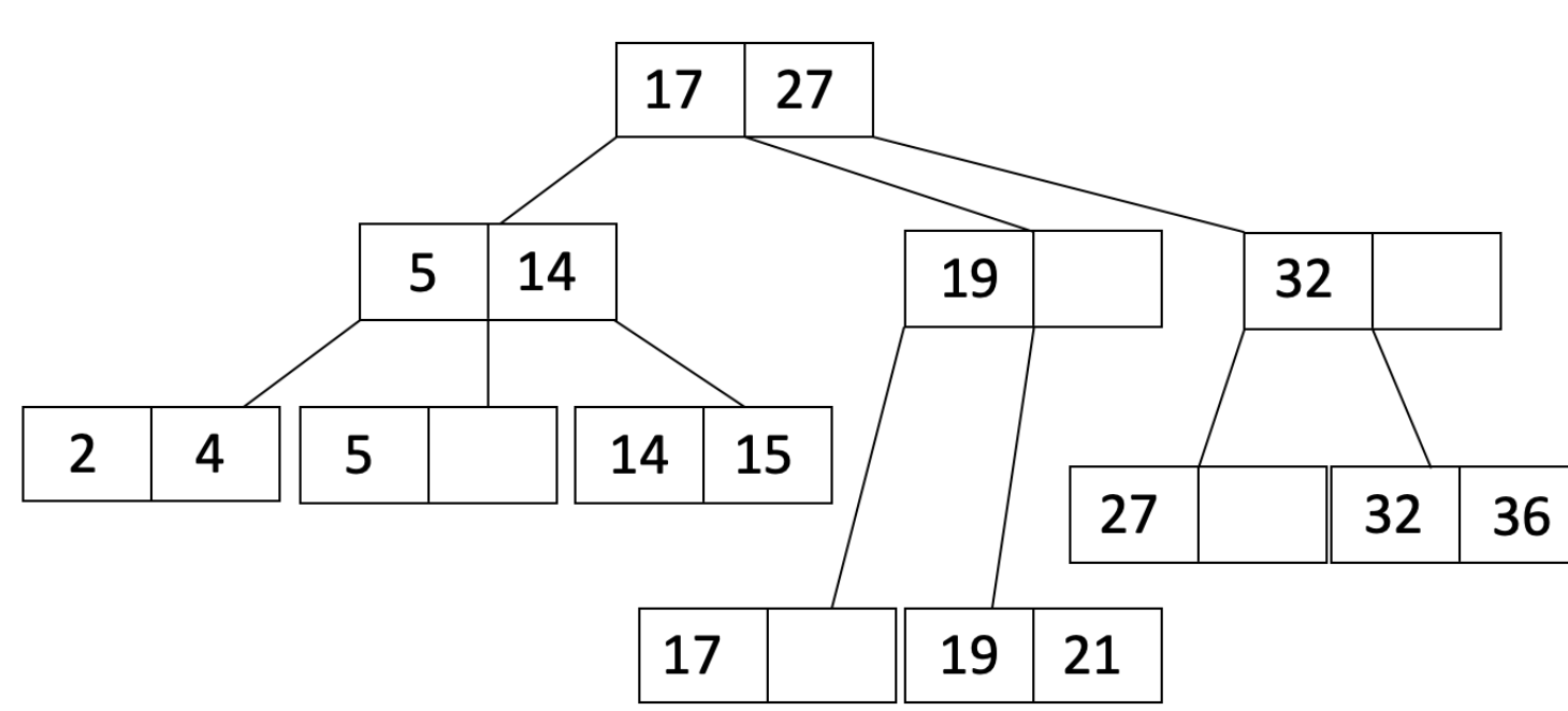
Let us try to demystify what indexes are, more than just “things” that make lookup faster. Indexes are just B Trees or B+ Trees that are added on top of the existing infrastructure that uses columns that uniquely identify records and use them as keys to create a B-Tree. Now a B Tree is simply a self-balancing tree that has multiple ordered children on each layer. This allows us to reach the leaves in logarithmic time. This is good for to lookup, insertion and deletion of these records. So one downside we can see right off the bat is that this setup will require more space, however, this downside often makes up for the performance benefits.

One question we need to answer is: What data are the leaves going to store? We have two possible answers to this question. One, they can store actual records themselves. Or two, they can store references to which page the record is stored on disk. The latter approach allows us to have multiple indexes on the file.

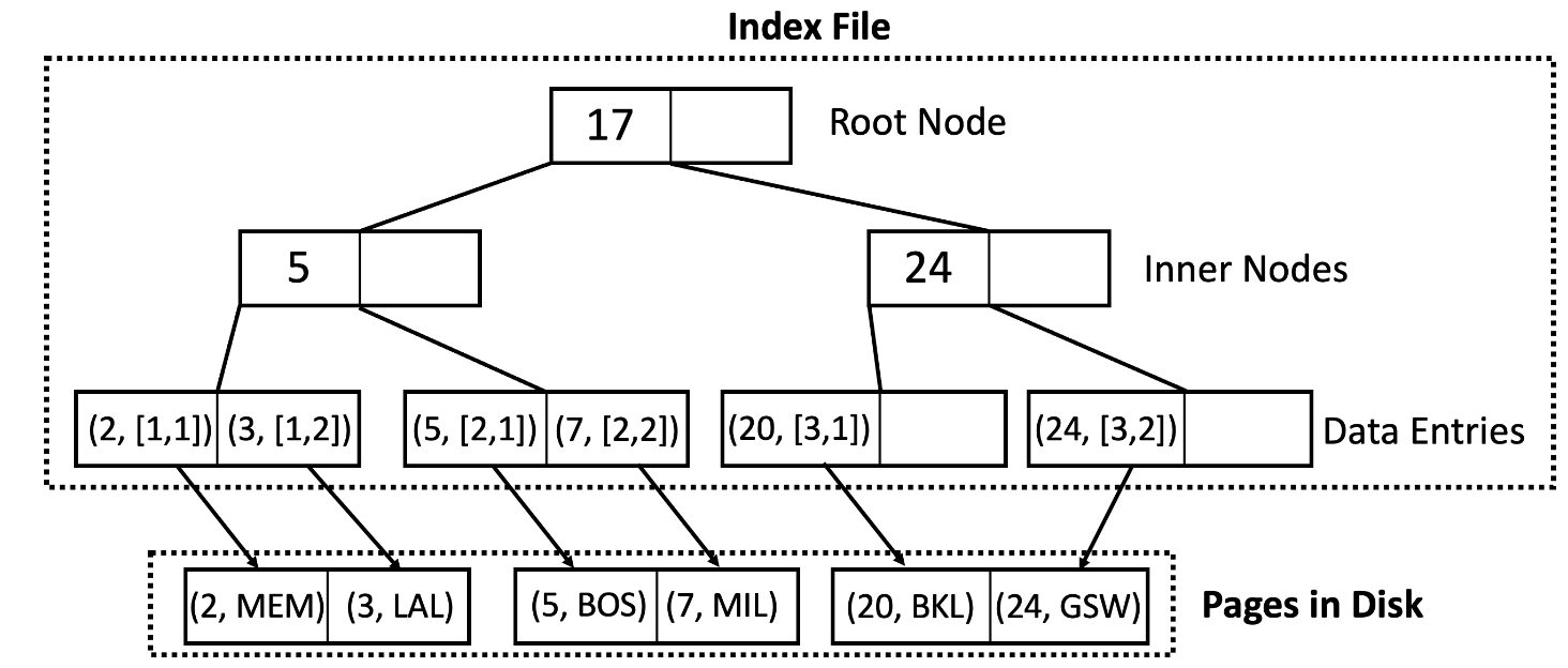
Now there is an important note to make on how data is clustered on disk. If the data is unclustered meaning that you can find one record on Page A and the adjacent record on Page B, this means will need to run through the index $n$ times for $n$ records since virtually no two records would ever be found on the same page. This is not optimal. A more optimal design would cluster adjacent records so that we can reduce the locality of data within pages and leverage the in-memory cache to store the page and use that same cache to retrieve the next record. This will save a lot more time.

Joins

Joins are arguably the most complex operations performed in a SQL query, let talk about how they are performed efficiently. There are two main ways to perform joins where SQL selects which algorithm to choose based on minimal I/O operations.

Index Nested Loop Join

When we are joining columns that happen to be indexes we can easily find the matching record. We go through the records in relation $R$ and use the index on the relation $S$ to find the matching record. We can then join these 2 records and add them to the resulting page in the buffer.

Hash Join

The problem with index join is that it still takes logarithmic time to find the target record. If we can find a way to leverage a hashmap we can potentially reduce the lookup to near constant time. Now we need to maximize the in-memory usage as a result we need to store as many pages as we can fit in-memory. If the buffer can store $B$ pages, we need to reserve one page for the resulting joined table and one page for relation $S$. That leaves us $B-2$ pages for relation $R$. Once we have these pages in memory we can create a hashmap for each record in $B-2$ pages. We can use this hashmap to find the matching records in $R$ by using hash keys generated from $S$.

Concurrency in SQL

Concurrecy in SQL is optimized through the use of two types of locks. Namely, exclusive locks (X-locks) and shared locks (S-locks). Exclusive locks are the same as what we learned from school, only one transaction has access to the resouce. For another transaction to get access, it will need to wait in a queue. The idea behind shared locks is that some transactions can be perfored at the same time. Specifically, read transaction can be performed at the same time since they do not mutate the data. Therefore, UPDATE, DELETE and INSERT naturally use the exclusive lock whereas all other transactions use the shared locks.

Although CONCURRENTLY is not a standard SQL keyword, it is heavily used in the creation of indexes. The idea behind this is to create an index without locking writes, updates and deletes to the table. This is means if write is performed while the index was being created, the index will automatically get updated for that record instead of blocking the write. Obviously this slows down the operation, however, for certain large tables this drawback is well worth the avaliablity.

DEADLOCKS

With heavy use of concurrency, deadlocks are a possibility. It occurs when two transactions have conflicting requests on resources. So for example, if transaction A has lock on resource A and is requesting access to resource B. While transaction B has lock on resource B and is requesting to resouce A. Not possible for both these transactions to move forward. Here is a good resource on avoiding deadlocks.

• ← Previous Post
• Next Post →