Contents
Overview
Machine Learning and AI is all the talk these days in engineering communities. AI in recent years achieved a great mile stone, it can now defeat any individual in any board game ever conceived by humans. Fully autonomous cars are coming closer reality with every passing year. So now is a good time as any to start to learn what is machine learning all about. The post will go through some of the core properties of neural networks such as Forward Propagation and Backward Propagation with some mathematical rigour.
This post will assume you have basic knowledge of Linear Algebra and Calculus.
What Is a Neural Network
A neural network is comprised of some number of layers, where each layer is comprised of some number of neurons. You may ask, what is a neuron?
Neuron
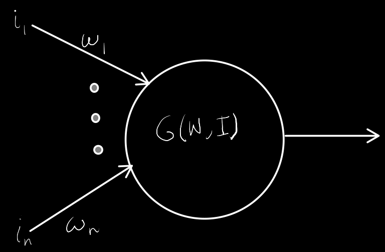
A neuron has the following structure:
 $$
\begin{aligned}
n &: \text{number of neurons on the previous layer} \newline
W &: \lbrack w_1, w_2 \dots w_n \rbrack \text{ weights from previous layer to this layer} \newline
I &: \lbrack i_1, i_2 \dots i_n \rbrack \text{ inputs from previous layer}\newline
\end{aligned}
$$
$G$ is a function that takes in $W$ and $I$ and determines if the neuron will fire. More precisely, we can define $G$ like so:
$$
\begin{equation}
G(W, I) = \sigma(W \cdot I)
\end{equation}
$$
So, $G$ performs a dot product between W and I, essentially taking a weighted sum of the previous layer: $w_1 \times i_1 + w_2 \times i_2 + \dots + w_n \times i_n$. This sum is then passed into the activation function $\sigma$, and then the activation function lets us know whether or not the neuron fired. A common activation function is the sigmoid:
$$
\sigma(x) = \frac{1}{1+e^{-x}}
$$
$$
\begin{aligned}
n &: \text{number of neurons on the previous layer} \newline
W &: \lbrack w_1, w_2 \dots w_n \rbrack \text{ weights from previous layer to this layer} \newline
I &: \lbrack i_1, i_2 \dots i_n \rbrack \text{ inputs from previous layer}\newline
\end{aligned}
$$
$G$ is a function that takes in $W$ and $I$ and determines if the neuron will fire. More precisely, we can define $G$ like so:
$$
\begin{equation}
G(W, I) = \sigma(W \cdot I)
\end{equation}
$$
So, $G$ performs a dot product between W and I, essentially taking a weighted sum of the previous layer: $w_1 \times i_1 + w_2 \times i_2 + \dots + w_n \times i_n$. This sum is then passed into the activation function $\sigma$, and then the activation function lets us know whether or not the neuron fired. A common activation function is the sigmoid:
$$
\sigma(x) = \frac{1}{1+e^{-x}}
$$
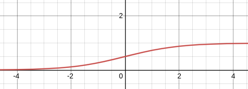
Note that the sigmoid function resembles the step function. If the sigmoid of the weighted sum is above $0.5$ then we can think of the neuron as firing. There are few important properties of the sigmoid function - it is differentiable, which is important for back propagation. It is bounded, it helps us determine which neurons have fired. There are several other types of activation functions each with their own set of benefits and drawbacks. For instance, it has been shown that the sigmoid some times leads to the Vanashing Gradient Problem which is detrimental for a neural networks ability to learn.
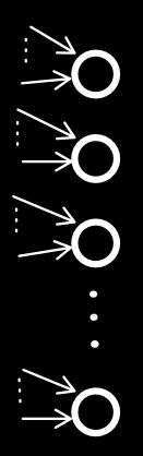
Layer of Neurons
It is exactly what it sounds like, a layer of neurons:
Neural Network
So finally a neural network is a set of layers:
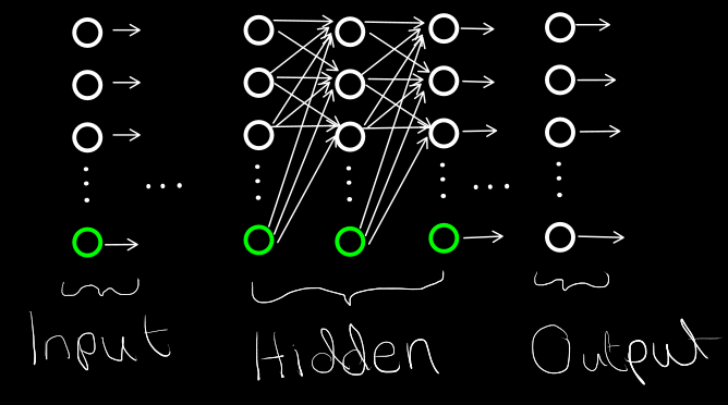
In a neural network, we usually have 3 types of layers. Input, hidden and Output layers. The input layers are responsible for supplying the subsequent hidden layer with inputs. The hidden layer is where all the magic happens, each neuron performs its function as defined above with the supplied inputs from the previous layer. The output layer gives the output of the neural network.
The Bias
You may have noted something weird about the image of the neural network above. Why aren’t the green neurons accepting any inputs? Well, they are special type of neurons called Bias neurons. Their speciality is that they always output a one.
Why do we need a bias neuron?
To understand why we need a bias neuron, we can run a thought experiment. Assume we build a neural network with 1 input neuron and 1 output neuron without any bias neurons and we adjust the weight from input to output such that for an input of $0$ we want an output of $0$. Assume we use a sigmoid activation function. The result of the output neuron will be so: $$ \begin{aligned} G(W, I) &= \sigma(w_1 \times 0) \newline &= 0.5 \end{aligned} $$ Note that no matter what we choose for $w_1$ we will always get an output of $0.5$ and so we can never teach the neural network to output a $0$. Now if we include a bias neuron, the result of the output neuron will be so: $$ \begin{aligned} G(W, I) &= \sigma(w_1 \times 0 + w_2 \times 1) \newline \end{aligned} $$ Now note that choose a sufficiently large negative value for $w_2$ will result in an output of close to $0$. Hence, the bias makes the neural network more powerful at learning.
Forward Propagation
To understand forward propagation we need mathematical notation for the entire network rather than just the neuron. Therefore we define the following variables: $$ W^{(l)} = \begin{bmatrix} w_{0,0}^{(l)} & \dots & w_{0,n}^{(l)} \newline \vdots & \ddots & \vdots \newline w_{m+1,0}^{(l)} & \dots & w_{m+1,n}^{(l)} \newline \end{bmatrix} $$
*Note that $^{(l)}$ not an exponent
We start by define $W^l \in \real^{m+1 \times n} $ where $w_{i. j}^l$ is the weight from the $i$-th neuron on layer $l-1$ to the $j$-th neuron on layer $l$. $$ I^{(1)} = \begin{bmatrix} i_0 \newline \vdots \newline i_m \end{bmatrix} $$ Next, we define the input vector at layer $1$, where $m$ input neurons are chosen for simplicity. In reality every layer could have an arbitrary number of neurons. Finally we define forward propagation from input layer to the first hidden layer as such: $$ \begin{equation} I^{(2)} = \sigma(I^{(1)T} \times W^{(2)})\newline \end{equation} $$
$$ I^{(2)}=\sigma\Bigg( \begin{bmatrix} i_0 \newline \vdots \newline i_m \newline 1 \end{bmatrix} ^ T \times \begin{bmatrix} w_{0,0}^{(1)} & \dots & w_{0,n}^{(1)} \newline \vdots & \ddots & \vdots \newline w_{m+1,0}^{(1)} & \dots & w_{m+1,n}^{(1)} \newline \end{bmatrix} \Bigg) $$
*Note that $^{T}$ is the transpose operation
So, the inputs to layer to can be computed as above. Each subsiquent layer can be computed in a similar way.
Backward Propagation
The purpose behind back-prop is to adjust the weights at each layer $W^{(l)}$ such that the output of the neural network $\bar{O}$ moves closer to the actual output $O$. To do so, we first must define the concept of error, a measure for how far $\bar{O}$ is from $O$. $$ \begin{equation} E = \frac{1}{2}\sum_{i=1}^{n}(o_i-\bar{o_i})^2 \end{equation} $$
$$ \text{Where $n$ is the number output of neurons} $$
We want to minimize $w_{i, j}^l$ such that the error is minimized. To do so, lets consider minimizing a simpler function: $$ f(x) = x^2 \newline \text{suppose we are currently at $x_o=-3$} $$ We can adjust the $x$ and move it in the direction of decreasing slope like so: $$ x_o = x_o - f’(x)\Bigr\rvert_{x=x_o}\newline~ \newline \text{Iteration 1:}\newline x_o = -3 - f’(x)\Bigr\rvert_{x=-3}\newline x_o = 3 \newline~ \newline \text{Iteration 2:}\newline x_o = 3 - f’(x)\Bigr\rvert_{x=3}\newline x_o = -3 $$ Hmm, looks like we aren’t making any progress:
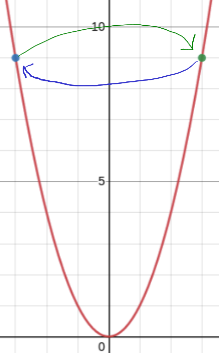
To fix this issue, we must add another a step size / learning rate $\alpha$ to ensure that each subsequent step is smaller than the previous. Suppose $\alpha = \frac{1}{3}$: $$ \begin{equation} x_o = x_o - \alpha f’(x)|_{x=x_o} \end{equation} $$
$$ \text{Iteration 1:}\newline x_o = -3 - \frac{1}{3}f’(x)|_{x=-3}\newline x_o = -1 $$
$$ \text{Iteration 2:}\newline x_o = -1 - \frac{1}{3}f’(x)|_{x=-1}\newline x_o = -1/3\newline \vdots $$
Now, we can see that $x_o$ is converging towards the minimum. This type of iterative optimization is referred to as Gradient Descent. The final tool we need to understand back-prop is the chain rule. Chain rule is a rule that defines derivatives of composition of functions.
$$ f(x) = y(g(x))\newline \frac{df}{dx} = \frac{dy}{dg}\frac{dg}{dx} $$ To understand why the chain rule is important we need view the output $\bar{O}$ as a compositions of outputs from previous layers.
$$ \begin{equation} \bar{O} = \sigma(\sigma(\sigma(… \times W^{(n-2)}) \times W^{(n-1)}) \times W^{(n)})\newline \end{equation} $$
Where $n$ is the total number of layers in the network
In order to update each weight, everytime we go back one layer we will need to use the chain rule to find the gradient that will minimize the error $E$ with respect to the weight $w_{i,j}^l$ . Once we have the gradient we need to update the weights according to equation (4). $$ \begin{equation} w_{i, j}^{(l)} = w_{i, j}^{(l)} - \alpha \frac{\partial E}{\partial w_{i, j}^{(l)}} \end{equation} $$