Contents
Overview
Dynamic Programming is a general technique for solving optimization, search, and counting problems that can be decomposed to subproblems. In such problems, these subproblems commonly reoccur and so we must cache the solutions to the subproblems and use them to solve larger problems until we obtain the solution to the original problem.
Introduction
Fibonacci Numbers
Let us start with a rather simple example, Fibonacci Numbers are computed using the following formula $F(n) = F(n-1) + F(n-2)$ and constructs the following infinite sequence $0, 1, 1, 2, 3, 5, 8, 13, 21, …$ Since the new element in the sequence is generated using the previous 2 elements suggests that Dynamic Programming can be leveraged. One observation to make is that the pattern cannot begin without base cases of $F(0) = 0$ and $F(1) = 1$. This is yet another manditory requirement of Dynamic Programming problems, we are to break a problem into subproblems, we require a base problem(s) or base case(s) to start constructing the solutions to larger problems till the original problem.
A naive approach utilizes recursion to solve the problem:
# Time: O(2^n) - Binary tree with height n & 2^n nodes
# Space: O(n)  - Stack space is the height of the tree, n
def Fib(n):
    if n == 0 or n == 1: return n
    return Fib(n-1) + Fib(n-2)
The following image shows the rescursion tree of computing Fib(6):
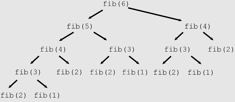
One thing to note is how in the recursion tree we are calling duplicate calls to
Fib. For example, Fib(3) is being called 3 times. We can use a hasmap to
temporary cache these results or we can use python’s built in @functools.lrucache
annotation to store intermediate results and thus avoid duplicate calls.
# Time: O(n) - duplicates will be cached and will not require recomputing
# Space: O(n) - The cache will still need to store n computations
@functools.lrucache()
def Fib(n):
    if n == 0 or n == 1: return n
    return Fib(n-1) + Fib(n-2)
Finally, we can use dynamic programming approach to construct the solution to
Fib(n). The approach is optimal as it only requires $O(1)$ space complexity:
# Time: O(n) - we need to solve n subproblems to reach and solve Fib(n)
# Space: O(1)
def Fib(n):
    if n == 0 or n == 1: return n
    fib_0, fib_1 = 0, 1
    for _ in range(1, n):
        fib_0, fib_1 = fib_1, fib_0 + fib_1
    return fib_1
Learnings:
Original problems can be solved easily once solutions to the subproblems are avaliable and cached
Maximum Subarray
Find the maximum subarray for a given array.
Example:
----------------------------------------------------------------------------------
|  A[0]  |  A[1]  |  A[2]  |  A[3]  |  A[4]  |  A[5]  |  A[6]  |  A[7]  |  A[8]  |
|--------|--------|--------|--------|--------|--------|--------|--------|--------|
|   904  |   40   |  523   |   12   | -335   | -385   | -124   |  481   |  -31   |
----------------------------------------------------------------------------------
We can start by constructing the brute force solution. We need two components for the brute force solution:
- We need a way to find a way to compoute
window_sum - We need a way to compute all possible subarrays
# Time: O(n) - from start to end, at worst end-start = n (size of array)
# Space: O(1)
def window_sum(array, start, end):
    sum = 0
    for idx in range(start, end):
        sum += array[idx]
    return sum

from math import inf

# Time: O(n^3) - 2 nested for loops, looping over array and call window_sum
# Space: O(1)
def maximum_subarray(array):
    max_sum = -inf
    for i in range(len(array)):
        for j in range(i+1, len(array)):
            max_sum = max(max_sum, window_sum(array, i, j)
    return max_sum
Before we continue to the Dynamic Programming solution, it is important to point out a time optimization at the cost of space complexity. We can precompute the following: $S[k] = \sum\limits_{k} A[0,k]$. $S$ now holds information to compute all window sums. The window sum for input array $A$ can be computed using the following formula $A[i,j] = S[j] - S[i-1]$ where $S[-1]$ is taken to be 0. This optimization could improve the time complexity to $O(n^2)$ at the cost of $O(n)$ space complexity.
Now, to solve this problem using dynamic programming, recall that the idea of dynamic programming is to use solutions to subproblems to construct the solution to the main problem. With this in mind, suppose we have the following array:
A = [2, 3, -2, 4]
We can assume A[0,0] is a subproblem, and within this subarray, the maximum
possible subarray is A[0], since it only contains one element. Now, we create a
larger subproblem by expanding the subarray to A[0, 1], and since the new element
increases the sum, it must be a part of the maximum subarray. We continue
enlarging the problem to A[0, 2]. In this case, we add a negative number to the
subproblem, so the maximum subarray remains the same. Finally, when we expand
to the original problem, we see that the maximum subarray is the subarray itself.
However, if we consider the case where $A[2] < -4$, we realize the final solution would have been different. To keep a running count of the maximum, we must condition on whether the newly added element is a good starting point for a new maximum subarray OR if it is negligible in the overall summation. With these insights, we can construct the following algorithm:
from math import inf

# Time: O(n) - running loop over the input array
# Space: O(1)
def maximum_subarray(array):
    running_max, current_max = -inf, -inf
    for element in array:
        running_max = max(element, running_max+element)
        current_max = max(current_max, running_max)
    return current_max
Tips for Dynamic Programming
- Consider using Dynamic Programming whenever you have to make choices to arrive at the solution
- Dynamic Programming can also be applicable when counting and decision problems
- Dynamic Programming often involves iteration or recusion along side taking advantage of a cache. The cache could be implmented as an 1-D or 2-D array, hash table or binary search tree.
- Array caches are often used for iterative solutions and hash tables or binary search trees are often used for recursive solutions
- Dynamic Programming is based on combining optimum solutions to subproblems to yield an optimum solution to the original solution
- IMPORTANT TIP When ever you construct a recursive solution is is very
important to ask, how would the space/time complexity change by simple caching
the function calls. I say this because often the difference between recursive
time complexity and DP time complexity can be achieved by using Python’s builtin
functools.lru_cache(None):
Ex: Counting Plays
Problem: In an American football game, a safety play leads to 2 points, a field goal leads to 3 points and a touchdown leads to 7 points. How many combinations of 2, 3 and 7 point plays can make up a final course.
We can start by implementing a brute force solution which creates a recursion tree branching on teach type of play that leads to points:
# Time: O(n^3) - function generates a 3-ary tree with max height of n
# Space: O(n) - the recursion stack height is n
# It is hard to pin point what n is but it is guranteed to be less that final_score
def play_possibilities(final_score):
    # Basecase
    if final_score == 0: return 1
    elif final_score < 0: return 0

    combinations = 0

    # safety
    combinations += play_possibilities(final_score - 2)
    # field goal
    combinations += play_possibilities(final_score - 3)
    # touchdown
    combinations += play_possibilities(final_score - 7)

   return combinations
With this nieve solution we see that this problems requires us to:
- Make choices
- Count
- Use recursion
Now to make use of these indicators to attempt a dynamic programming solution, we first must identify sub problems and how to use the solutions of the sub problems to construct the solution the main problem. To find the total combination of 2,3,7 plays to reach a particular score. We can ask the following sub questions:
- how many combinations to abtain a final score of
final_score-1? - how many combinations to obtain a final score only using 2,3 point plays?
These sub problems give us a mental model of the type of data structure that will come in handy:
   0   1   2   3   ...   n  <- score
+---+---+---+---+---+---+
| 1 |   |   |   |   |   | <- 2 points
+---+---+---+---+---+---+
| 1 |   |   |   |   |   | <- 2,3 points
+---+---+---+---+---+---+
| 1 |   |   |   |   |   | <- 2,3,7 points
+---+---+---+---+---+---+
Note we do not need any points to react a score of 0. Its a base case.
Now lets move on to the next question, how can we use the solutions to these
sub problems to solve “the problem”. To figure this out, lets complete the
datascructure with an example of final_score=10.
   0   1   2   3   4   5   6   7   8   9  10  <- score
+---+---+---+---+---+---+---+---+---+---+---+
| 1 | 0 | 1 | 0 | 1 | 0 | 1 | 0 | 1 | 0 | 1 | <- 2 points
+---+---+---+---+---+---+---+---+---+---+---+
| 1 | 0 | 1 | 1 | 1 | 1 | 2 | 1 | 2 | 2 | 3 | <- 2,3 points
+---+---+---+---+---+---+---+---+---+---+---+
| 1 | 0 | 1 | 1 | 1 | 1 | 2 | 1 | 2 | 2 | 4 | <- 2,3,7 points
+---+---+---+---+---+---+---+---+---+---+---+
Lets define this data structure as $A$ with indicies $i, j$. As we traverse
$A$, horizontally we must determine if that score is reachable using the current
row points, say $p$. This can be done by the following update:
$$ A[i, j] = A[i, j-p] $$
This will hit the base case at index 0, which will determine if the current $j$ is a multiple of the current point. If it is this score is reachable using a multiple of the current point
Now as we traverse $A$ vertically, we must determine how many solutions can be obtained using the points from the previous row. Thus, we can derive the following update rule:
$$ A[i, j] = A[i-1, j] $$ Together, these update rules account for existing possibilities from the previous row and new possibilities from the current row. Giving the final, all accounting update rule:
$$ A[i, j] = A[i, j-p] + A[i-1, j] $$
These rules can be implemented using python as such:
# Time: O(sn)
# Space: O(sn)
# Where s is the # of possible play scores (3 in this case)
# And n is the final_score
def play_possibilities(final_score):
    dp_solutions = [[1]+[0] * final_score for _ in range(3)]
    play_score = [2, 3, 7]
    for play in range(3):
        for score in range(final_score+1):
           existing_possibilities = dp_solutions[play-1][score] if play > 0 else 0
           new_possibilities = dp_solutions[play][score - play_score[play]] \
                if score >= play_score[play] else 0
           dp_solutions[play][score] = existing_possibilities + new_possibilities
    return dp_solutions[-1][-1]
Now if you recall the important tip from the tips section, we can simply cache the function calls, and believe it or not, we again reach the optimal solution once again:
import functools

# Time: O(n) - the function is called at most n times due to memoization
# Space: O(n) - the cache size to store memoized results
# n is the final_score
@functools.lru_cache(None)
def play_possibilities(final_score):
    # Basecase
    if final_score == 0: return 1
    elif final_score < 0: return 0

    combinations = 0

    # safety
    combinations += play_possibilities(final_score - 2)
    # field goal
    combinations += play_possibilities(final_score - 3)
    # touchdown
    combinations += play_possibilities(final_score - 7)

    return combinations
Memoizing / Caching is very powerful to optimize recursive solutions!
Ex: Leveshtein Distance
Levenshtein Distance: The minimum number of edits that it takes to transform from one word to another. Where edits are one of the following:
- Insertion: Inserting one character
- Deletion: Removing one character
- Substitution: Exchanging one character for another
Write a program that takes two strings and computes the minimum levenshtein Distance.
Lets begin by trying to understand how to solve the brute force, nieve solution. Given 2 words, $A$ and $B$, we want to write a function $E$ which computes minimum cost of converting string $A$ into string $B$ using the above 3 rules. Applying each rule will require a cost of 1.
To develop a brute force solution, we can use a recursive approach that breaks down the problem into smaller problems. Specifically, lets compare the 2 strings character by character and make one of three edits (or all 3 edits), insertion, deletion and substitution. All the while computing cost of each possibility.
We can define our function $E(i, j)$ where $i$ and $j$ are the indices of characters in strings $A$ and $B$ respectively. Since we are using recursion we need to start by identifying base cases:
- If $i$ is equal to the length of $A$ but $j$ is not the end of $B$, this means the remaining characters must be deleted so the cost is effectively $|B| - j$.
- Conversely, if $j = |B|$ then the cost is $|A| - i$.
Now, need to understand how exactly, the recursion will take place. Recursion typically results in various branches on each level. The branching factor for Fibonacci is $2$. For this problem, it makes sense to branch on each particular type of edit since we are not sure which one will result in minimum possible distance:
- Insertion: We skip one character in $B$ and add one to the cost. This simulates us inserting a character of our choice and is equivalent to calling $E(i, j + 1) + 1$. Where the $+1$ accounts for the accrued cost due to the edit.
- Deletion: We skip one character in $A$ and add 1 to the cost. This effectively simulates us deleting the skipped character and is equivalent to calling $E(i + 1, j) + 1$.
- Substitution: We compare both characters at positions $i$ and $j$, if they match then we increment both pointers and add a cost of 0. Otherwise, we again increment but add a cost of 1. This simulates substituting a character in either $A$ or $B$ (doesn’t matter which). This is equivalent of $E(i+1, j+1) + (0 \text{ or } 1)$.
Finally, we can take the minimum of these 3 values to obtain the smallest total cost over all levels of the recursion tree.
# Time: O(3 ^ min(len(A), len(B))) - 3 branches, height of min(len(A), len(B))
# Space: O(min(len(A), len(B))) - Recursion stack size
def levenshtein_distance(A, B, i=0, j=0):
    # Basecases
    if len(A) == i: return len(B)-j
    if len(B) == j: return len(A)-i

    # Compute cost
    cost = 0 if A[i] == B[j] else 1

    # min( Insertion, Deletion, Substitution )
    return min(
        levenshtein_distance(A, B, i, j+1) + 1, # Insert char in A
        levenshtein_distance(A, B, i+1, j) + 1, # Delete char in A
        levenshtein_distance(A, B, i+1, j+1) + cost, # Substitute matching char
    )
This thought process should be shouting Dynamic programming due to the simple fact that question requiring:
- Choices between insertion, deletion and substitution, i.e decision problem
- Use of recursion and solution to subproblems for the final solution
Lets use the important tip from the tips section and simply cache the function calls:
# Time:  O(len(A) * len(B)) - len(A) options for i, len(B) options for j then the cache will be filled for all subproblems
# Space: O(min(len(A)), len(B)) - Recursion stack size
@functools.lru_cache(None)
def levenshtein_distance(A, B, i=0, j=0):
    # Basecases
    if len(A) == i: return len(B)-j
    if len(B) == j: return len(A)-i

    # Compute cost
    cost = 0 if A[i] == B[j] else 1

    # min( Insertion, Deletion, Substitution )
    return min(
        levenshtein_distance(A, B, i, j+1) + 1, # Insert char in A
        levenshtein_distance(A, B, i+1, j) + 1, # Delete char in A
        levenshtein_distance(A, B, i+1, j+1) + cost, # Substitute matching char
    )
This is as optimal as the DP solution, in fact it is more optimal since the
dynamic programming solution requires len(A) * len(B) space complexity.
Here are the functions timed:
Original Execution time: 0.011868 seconds
Cached Execution time: 0.000072 seconds
If you were to write a DP solution that avoids recursion and @functools.lru_cache(None),
you would get the same time complexity. However, lets work through it for the sake
of it. We will need to create a data structure that allows us to compute cost for
strings A and B. Lets again go with a 2D matrix, where the rows are
the characters of string $A$ and columns are characters of string $B$ and the cells[i][j]
are the costs to convert A[0:i] to B[0:j] or vise versa.
For example, let $A$ be kitten and $B$ be sitting:
         ""  "k" "i" "t" "t" "e" "n"
   ""     .   .   .   .   .   .   .
   "s"    .   .   .   .   .   .   .
   "i"    .   .   .   .   .   .   .
   "t"    .   .   .   .   .   .   .
   "t"    .   .   .   .   .   .   .
   "i"    .   .   .   .   .   .   .
   "n"    .   .   .   .   .   .   .
   "g"    .   .   .   .   .   .   .
Note: using empty strings are very important to establish the base case
The base cases are rather straight forward, since it takes k insertions to go
from "" to A[:k] or B[:k].
         ""  "k" "i" "t" "t" "e" "n"
   ""     0   1   2   3   4   5   6
   "s"    1   .   .   .   .   .   .
   "i"    2   .   .   .   .   .   .
   "t"    3   .   .   .   .   .   .
   "t"    4   .   .   .   .   .   .
   "i"    5   .   .   .   .   .   .
   "n"    6   .   .   .   .   .   .
   "g"    7   .   .   .   .   .   .
Now every other combination of $i$ and $j$ must be computed specifically to minimize the cost using the optimal decision between insertion, deletion and substitution. For this solution, I claim the following formula is correct:
dp[i][j] = min(dp[i-1][j-1] + {0, 1}, dp[i-1][j] + 1, dp[j-1][i] + 1)
The first part, dp[i-1][j-1]+{0,1} accounts for the cost required for
substitution. If the A[i] == B-[j] then we add $0$ to the previous diagonal
otherwise we add $1$. The dp[i-1][j] can be thought of as deleting i-th
character in $A$ and adding $1$ for the cost. The dp[i][j-1] can be thought of
as inserting the j-th character from $B$ into $A$ amd we again add $1$ for the
cost.
# Time: O(len(A) * len(B)) - the 2 for loops
# Space: O(len(A) * len(B)) - size of dp
def levenshtein_distance(A, B):
    dp = [[0] * (len(B) + 1) for _ in range(len(A) + 1)]

    for i in range(len(A) + 1):
        for j in range(len(B) + 1):
            if i == 0 or j == 0:
                dp[i][j] = max(i, j)
            else:
                cost = 0 if A[i-1] == B[j-1] else 1
                dp[i][j] = min(dp[i-1][j-1]+cost, d[i-1][j]+1, dp[i][j-1]+1)

    return dp[len(A)][len(B)]
Ex: Counting ways to traverse a 2D array
Wriate a program that counts how many ways you can go from the top left to the bottom right in a $n$ by $n$ 2D array. For example:
+-+-+-+-+-+-+
|→|→|→|→|→| |
+-+-+-+-+-+-+
| | | | |↓| |
+-+-+-+-+-+-+
| | | | |↓| |
+-+-+-+-+-+-+
| | | | |↓| |
+-+-+-+-+-+-+
| | | | |↓|→|
+-+-+-+-+-+-+
Lets follow the same recepie layed out in previous examples. Lets start by thinking of a recursive solution. In this case, we have 2 possible decisions:
- Move Right
- Move Down
Now lets define a base case, if we reach cell in grid[n-1][n-1] we return $1$.
Otherwise, if we exceed the boundaries, we return 0. We can accrue the count for
the final result. Now we have enough information to solve the problem:
# Time: O(2 ^ n) - Decision tree has 2 branches that can each go at most n deep
# Space: O(n ^ 2) - Stack space can go at most n * n deep
def traversal_count(n, i=0, j=0):
    # Basecase
    if i < 0 or i >= n: return 0
    if j < 0 or j >= n: return 0
    if i==n-1 and j == n-1: return 1

    # Compute Total Ways
    return traversal_count(n, i+1, j) + traversal_count(n, i, j+1)
Lets take advantage of our important tip, and cache the function calls to ensure they are only called once:
# Time: O(n ^ 2) - n options for i and n options for j at most nxn possible options
# Space: O(n ^ 2) - Stack space can go at most n * n deep
@functools.lru_cache(None)
def traversal_count(n, i=0, j=0):
    # Basecase
    if i < 0 or i >= n: return 0
    if j < 0 or j >= n: return 0
    if i==n-1 and j == n-1: return 1

    # Compute Total Ways
    return traversal_count(n, i+1, j) + traversal_count(n, i, j+1)
See how it becomes easier and easier to reach the optimal solution if you follow the same recepie. Going through these recursive optimizations clears out a path towards approaching the iterative solution and often coming up with the iterative solution is harder.
Now following the previous patterns, we know that we will need an n by n array
which in each cell stores the number of ways to reach that cell. As for the
base case, we know the first row and column are only reachable in $1$ way.
Going fully right or fully down. We know the formula to compute the number of ways
will be related to the recursive model. However, if we reason though the thought
process we realize that to reach a cell $(i,j)$ we could have either gone up or
to the right. So, dp[i][j] = dp[i-1][j] + dp[i][j-1]. So we have the following
formula:
# Time: O(n ^ 2) - 2 for loops of range n
# Space: O(n ^ 2) - 2D array of size n by n
def traversal_count(n):
    dp = [[0] * n for _ in range(n)]
    for i in range(n):
        for j in range(n):
            if i==0 or j==0: dp[i][j] = 1
            else:
                dp[i][j] = dp[i-1][j] + dp[i][j-1]
    return dp[n-1][n-1]
Ex: Compute Binomial Coefficients
The binomial theorm is used to determine the number of ways to choose k elements from n elements: $$ \binom{n}{k} = \frac{n!}{k!(n-k)!} $$ Note that direct computation of this formula results in numerator and denominator overflow because the values grow very fast. Even if the final result fits as a 32-bit integer. Design an efficient algorithm for computing $\binom{n}{k}$ which has a property that it never overflows if the final results fits in the integer word size.
Lets start by understanding the brute force approach of the binomial algorithm. We can write a factorial function to compute $n!$, $k!$ and $(n-k)!$.
# Time: O(n) - We have to call the factorial n times
# Space: O(n) - Stach space of size n
def factorial(n):
    if n==0: return 1
    return n * factorial(n-1)

# Time: O(max(n, k))
# Space: O(max(n, k))
def binomial(n, k):
    return factorial(n) / (factorial(k) * factorial(n-k))
We could of course optimize the program by caching the function calls on factorial. However, this does not effect the complexity:
# Time: O(n) - We have to call the factorial n times
# Space: O(n) - Stach space of size n
@functools.lru_cache(None)
def factorial(n):
    if n==0: return 1
    return n * factorial(n-1)

# Time: O(max(n, k))
# Space: O(max(n, k))
def binomial(n, k):
    return factorial(n) / (factorial(k) * factorial(n-k))
However, the issues with these neive implementations is that they quickly run into overflow issues even if the final result does not consist of an overflow. To avoid overflow issues we must take advantage of a particular property of the binomial theorm:
$$ \binom{n}{k} = \binom{n-1}{k-1} + \binom{n-1}{k} $$
This now requires us to perform significantly smaller factorial calculations, thus allowing us to compute larger binomial coefficients.
Additionally, in the notation alone we note the recursive nature of this property. In other words, to compute a binomial coefficient, we must compute $2$ smaller coefficients. We note that we keep replacing the binomials with smaller and smaller summations. Eventually we reach $k=0$ which becomes the base case because $\binom{n}{0}=1$. We also know $\binom{n}{n}=1$. These become the base cases (one for each term, one where $n$ is decreasing to $k$ and another where $k$ is decreasing to $0$).
# Time: O(2 ^ (n + k)) -first term of the property goes to a depth of k
#                       and second term goes to a depth of n. Total worst case
#                       depth is n + k
# Space: O(n + k)      -again worst case depth is n + k
def binomial(n, k):
    # Basecase
    if k == 0 or k == n: return 1

    # Use binomial property
    return binomial(n-1, k) + binomial(n-1, k-1)
Lets take advantage of our important tip and mitigate the exponential complexity.
# Time: O(n + k) - first term of the property goes to a depth of k
#                       and second term goes to a depth of n. Total worst case
#                       depth is n + k
# Space: O(n + k) - again worst case depth is n + k
@functools.lru_cache(None)
def binomial(n, k):
    # Basecase
    if k == 0 or k == n: return 1

    # Use binomial property
    return binomial(n-1, k) + binomial(n-1, k-1)
Boom! Best case time and space complexities. Now lets go through the iterative solution for the practice. Plus, the iterative solution unravels alot of the information needed to write the iterative solution. As before, the base cases are the same and we are using 2D array in which we can compute $\binom{n}{k}$ along with all its sub problems.
+---+---+---+---+---+---+---+
|   | 0 | 1 | 2 | 3 |...| k |
+---+---+---+---+---+---+---+
| 0 |   |   |   |   |   |   |
+---+---+---+---+---+---+---+
| 1 |   |   |   |   |   |   |
+---+---+---+---+---+---+---+
| 2 |   |   |   |   |   |   |
+---+---+---+---+---+---+---+
| 3 |   |   |   |   |   |   |
+---+---+---+---+---+---+---+
|...|   |   |   |   |   |   |
+---+---+---+---+---+---+---+
| n |   |   |   |   |   |   |
+---+---+---+---+---+---+---+
# Time: O(n * k) - 2 for loops of size n and k
# Space: O(n * k) - n * k 2D array
def binomial(n, k):
    dp = [[0] * k+1 for _ in range(n+1)]

    for i in range(n+1):
        for j in range(k+1):
            if j == 0 or i == n: dp[i][j] = 1
            else:
                dp[i][j] = dp[i-1][j] + dp[i-1][j-1]

    return dp[n][k]
We can make a small optimization to avoid computing unnecessary values:
# Time: O(n * min(k, n - k))
# Space: O(n * k)
def binomial(n, k):
    dp = [[0] * (k+1) for _ in range(n+1)]

    for i in range(n+1):
        for j in range(min(i, k) + 1):
            if j == 0 or i == j: dp[i][j] = 1
            else:
                dp[i][j] = dp[i-1][j] + dp[i-1][j-1]

    return dp[n][k]
Oddly enough the iterative solution does not perform better than the memoized recursive solution.
Ex: Search for a sequence in a 2D Array
Lets move on to bit of a more unique problem, which may sound hard at first but we will break it down step by step.
Suppose you have a 2D array of integers such as the following:
| 1 2 3 |
| 3 4 5 |
| 5 6 7 |
And a 1D array, we will refer to this as the pattern:
| 1 |
| 3 |
| 4 |
| 6 |
We say the the pattern occurs in the 2D grid if we can start at some entry of the grid and traverse adjacent entries in the order that is specified by the pattern till all entries in the pattern have been visited. It is acceptable for you to visit the same entry more than once as long as the entries are adjacent.
# Time: O(4^max(mn, p)) - We have 4 recursive branches & max height of max(mn,p)
# Space: O(max(mn,p)) - max height of max(mn,p)
# Let the size of grid be mxn
# Let the size of the pattern be p
def is_pattern_in_grid( grid, pattern, row=0, col=0, pattern_idx=0 ):
    row_len, col_len, pattern_len = len(grid), len(grid[0]), len(pattern)

    # Basecases
    if pattern_idx == pattern_len: return True
    if row < 0 or row >= row_len: return False
    if col < 0 or col >= col_len: return False

    # Increment pattern position
    if pattern[pattern_idx] == grid[row][col]: pattern_idx += 1

    # Left, Right, Up, Down Traversal
    return  is_pattern_in_grid( grid, pattern, row+1, col, pattern_idx) or \
            is_pattern_in_grid( grid, pattern, row-1, col, pattern_idx) or \
            is_pattern_in_grid( grid, pattern, row, col+1, pattern_idx) or \
            is_pattern_in_grid( grid, pattern, row, col-1, pattern_idx)
Lets take advantage of our important tip and memoize the function call to
avoid duplicate (row, col, pattern_idx) calls:
# Time: O(mnp) - all possible combinations of (row,col,pattern_idx)
# Space: O(max(mn,p)) - max height of max(mn,p) is still the same
# Let the size of grid be mxn
# Let the size of the pattern be p
@functools.lru_cache(None)
def is_pattern_in_grid( grid, pattern, row=0, col=0, pattern_idx=0 ):
    row_len, col_len, pattern_len = len(grid), len(grid[0]), len(pattern)

    # Basecases
    if pattern_idx == pattern_len: return True
    if row < 0 or row >= row_len: return False
    if col < 0 or col >= col_len: return False

    # Increment pattern position
    if pattern[pattern_idx] == grid[row][col]: pattern_idx += 1

    # Left, Right, Up, Down Traversal
    return  is_pattern_in_grid( grid, pattern, row+1, col, pattern_idx) or \
            is_pattern_in_grid( grid, pattern, row-1, col, pattern_idx) or \
            is_pattern_in_grid( grid, pattern, row, col+1, pattern_idx) or \
            is_pattern_in_grid( grid, pattern, row, col-1, pattern_idx)
Now, the iterative solution does not involve DP (or atleast I can’t think of an iterative DP solution). So we’ll skip the iterative solution for the sake of staying on topic.